In the notes for this week, I highlighted the importance of data preparation in the overall ML process. We’ve covered most of these in previous weeks, but they are worth revising as they are critical not only for effective ML analysis, but for general statistical analysis.
72.2 Handling missing values
Theory
Handling missing values is crucial in ML to maintain the integrity and accuracy of our models. As you know, missing data can occur for various reasons, such as errors in data entry, non-response in surveys, or interruptions in data collection.
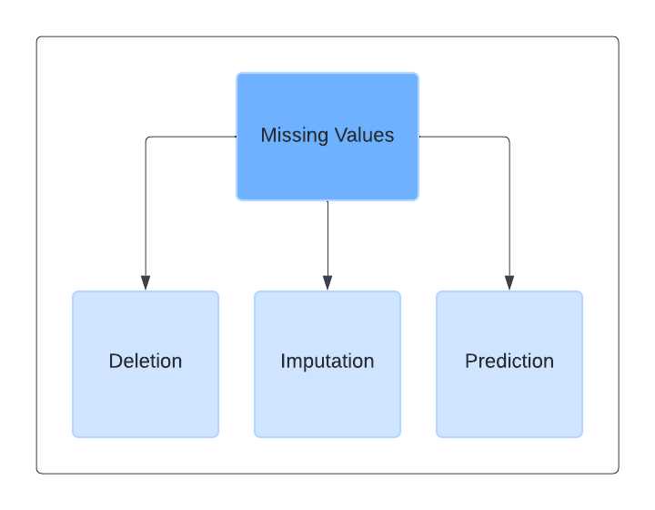
There are three strategies to manage missing values, each with its advantages and limitations:
Removal: This method involves deleting rows (observations) or columns (variables) with missing values. It’s straightforward, but can lead to a significant reduction in data size and potential bias if the missing values are not random.
Imputation: Imputation fills in missing values with estimates based on the rest of the available data. Common methods include using the mean, median, or mode of the column.
Prediction: More advanced than simple imputation, prediction models use machine learning algorithms to estimate missing values based on patterns found in other variables.
Removal: demonstration
The task is to clean a dataset of athlete performances by removing records with missing values.
Rather than simply deleting observations with missing values, a more sophisticated strategy is to impute missing values.
For example, in the dataset marathon-data, I could deal with missing values through median imputation (taking the middle value for the variable and inserting it into the missing values).
set.seed(123)# Generate synthetic datarunner_id <-1:100finish_time <-rnorm(100, mean =240, sd =20)# Introduce missing valuessample_indices <-sample(1:100, 20)finish_time[sample_indices] <-NA# Combine into a data framemarathon_data <-data.frame(runner_id, finish_time)# Calculate the median of the available finish timesmedian_time <-median(marathon_data$finish_time, na.rm =TRUE)# Impute missing finish times with the median valuemarathon_data$finish_time[is.na(marathon_data$finish_time)] <- median_time# Verify imputationhead(marathon_data)
A third strategy, which is (usually) even better, is to use predictive modeling to predict what the missing value might be.
For example, we can create a regression model for the variable that has missing values, and use that model to generate predicted values:
set.seed(123)# Generate synthetic data for cricket playersplayer_id <-1:100# 100 playersbatting_average <-round(rnorm(100, mean =35, sd =5),1)bowling_average <-round(rnorm(100, mean =25, sd =3),1)sample_indices <-sample(1:100, 20)bowling_average[sample_indices] <-NA# Combinecricket_data <-data.frame(player_id, batting_average, bowling_average)# Split data into sets with known and unknown bowling averagesknown_bowling <- cricket_data[!is.na(cricket_data$bowling_average), ]unknown_bowling <- cricket_data[is.na(cricket_data$bowling_average), ]# Build model to predict bowling_average using batting_average from the known datasetmodel <-lm(bowling_average ~ batting_average, data = known_bowling)# Predict the missing averagespredictions <-predict(model, newdata = unknown_bowling)# Replace missing values with predictionscricket_data$bowling_average[is.na(cricket_data$bowling_average)] <- predictions# Verify predictionsprint("Data after Predicting Missing Values:")
Outlier detection is another vital step in preparing data for ML.
It aims to identify and possibly exclude data points that significantly differ from the majority of the dataset. These points can be due to variability in the measurement or potential measurement error. In the context of sport analytics, outliers might represent extraordinary performances or (more likely) data entry errors.
We’ve discussed this before, but a reminder that there are several methods available to detect outliers, including:
Statistical Methods: Using standard deviation and z-scores to find points far from the mean.
Interquartile Range (IQR): Identifies outliers as data points that fall below the 1st quartile minus (1.5 times * IQR) or above the 3rd quartile plus (1.5 times * IQR).
Boxplots: Visually inspecting for points that fall outside the ‘whiskers’ in a boxplot can also help identify outliers.
Identifying outliers: demonstration
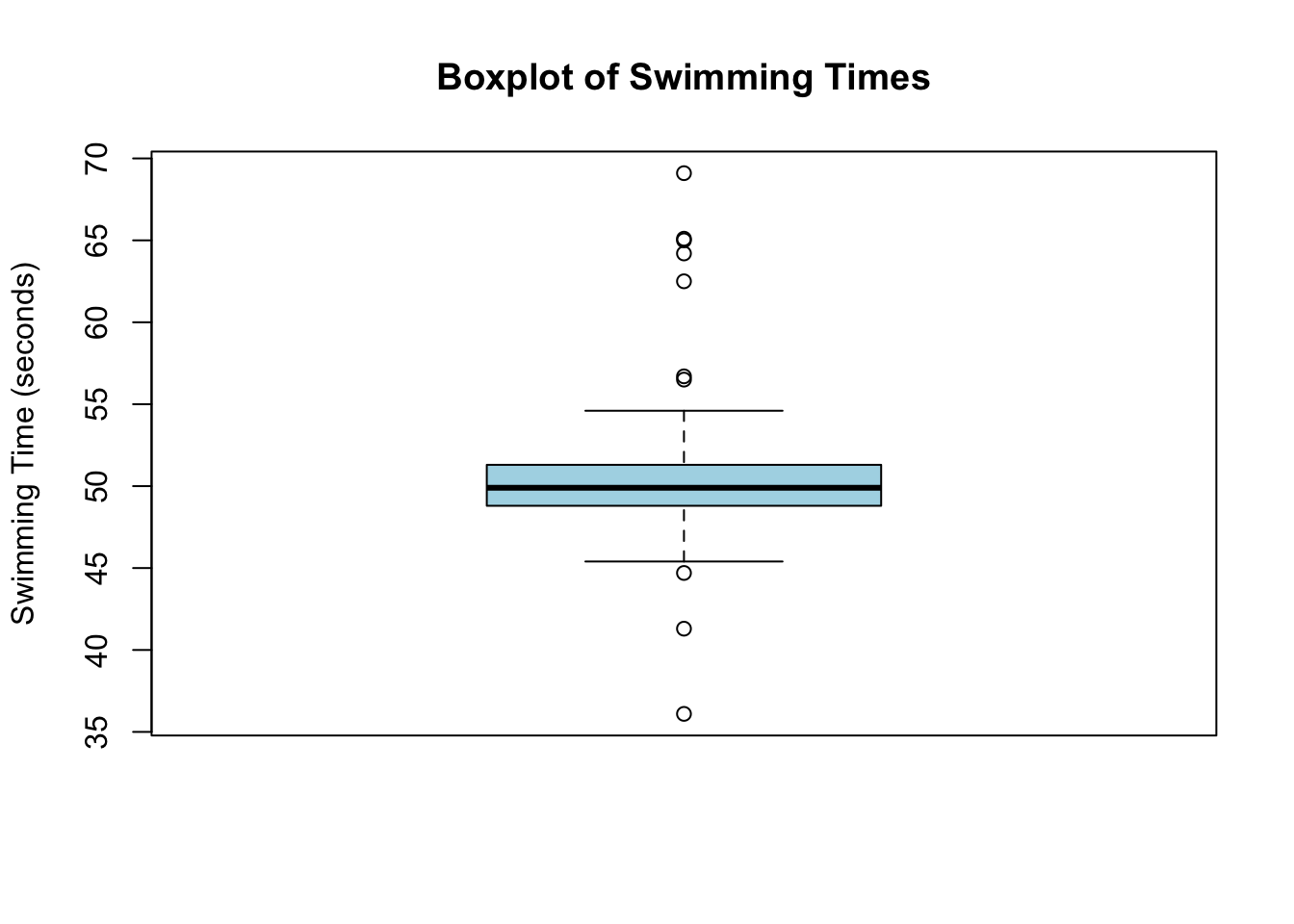
Identify and analyse outliers in a dataset of Olympic swimming times.
set.seed(123)swimming_data <-data.frame(athlete_id =1:300,swimming_time =c(rnorm(290, mean =50, sd =2), runif(10, min =30, max =70)) )swimming_data$swimming_time <-round(swimming_data$swimming_time,1)# visually inspect outliersboxplot(swimming_data$swimming_time, main ="Boxplot of Swimming Times",ylab ="Swimming Time (seconds)", col ="lightblue")
Once outliers have been identified in a dataset, the next step is to decide how to deal with them. Our approach to dealing with outliers depends on their nature, and the context of the study.
Here’s a reminder of some common strategies:
Exclusion: Removing outliers if they are determined to be due to data entry errors or if they are not relevant to the specific analysis.
Transformation: Applying a mathematical transformation (such as log transformation) to reduce the impact of outliers.
Imputation: Replacing outliers with estimated values based on other data points.
Separate Analysis: Conducting analyses with and without outliers to understand their impact.
Dealing with outliers: demonstration (2)
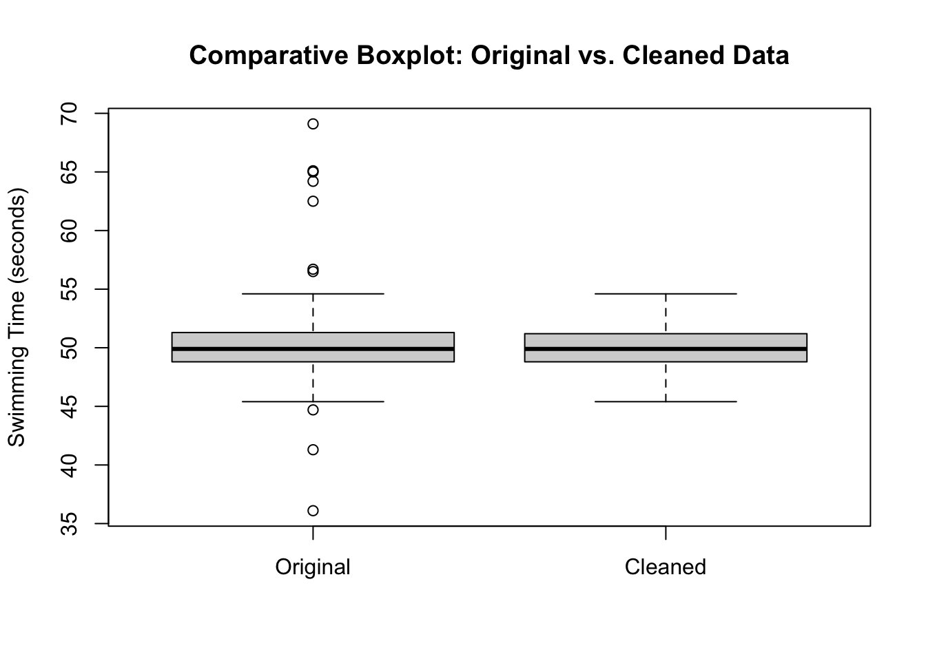
We can analyse the effect of outliers in the Olympic swimming times dataset and apply a method like exclusion to deal with them.
# olympic_swimming_data with identified outliers# Analysing the impact of outlierssummary(swimming_data$swimming_time)
   Min. 1st Qu.  Median    Mean 3rd Qu.    Max.
  36.10   48.80   49.90   50.22   51.30   69.10
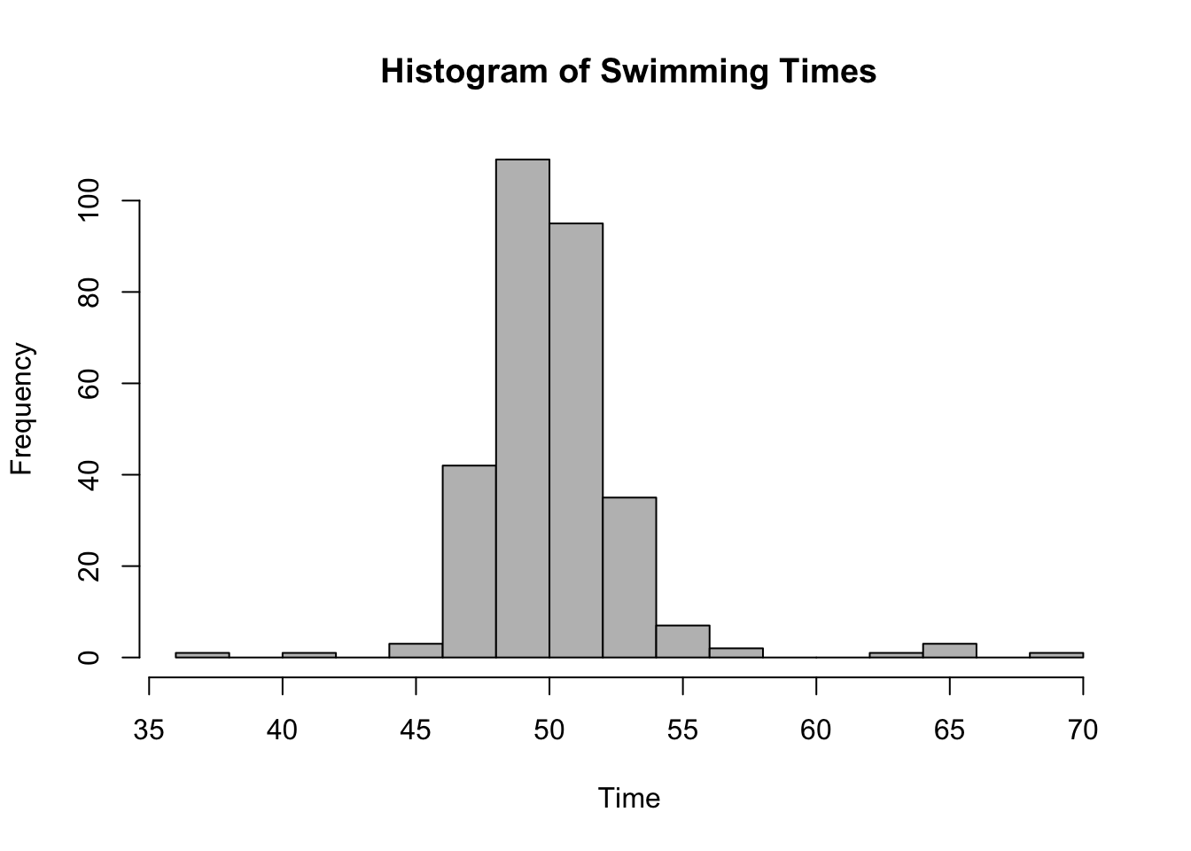
hist(swimming_data$swimming_time, main ="Histogram of Swimming Times", xlab ="Time", breaks =20, col ="gray")
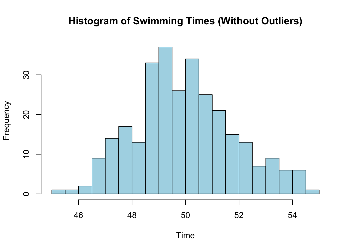
# I'll exclude the outlierscleaned_data <- swimming_data[!(swimming_data$swimming_time < lower_bound | swimming_data$swimming_time > upper_bound), ]# Re-analyse without outlierssummary(cleaned_data$swimming_time)
   Min. 1st Qu.  Median    Mean 3rd Qu.    Max.
  45.40   48.80   49.90   50.02   51.20   54.60
hist(cleaned_data$swimming_time, main ="Histogram of Swimming Times (Without Outliers)", xlab ="Time", breaks =20, col ="lightblue")
# Compare resultsboxplot(swimming_data$swimming_time, cleaned_data$swimming_time,names =c("Original", "Cleaned"),main ="Comparative Boxplot: Original vs. Cleaned Data",ylab ="Swimming Time (seconds)")
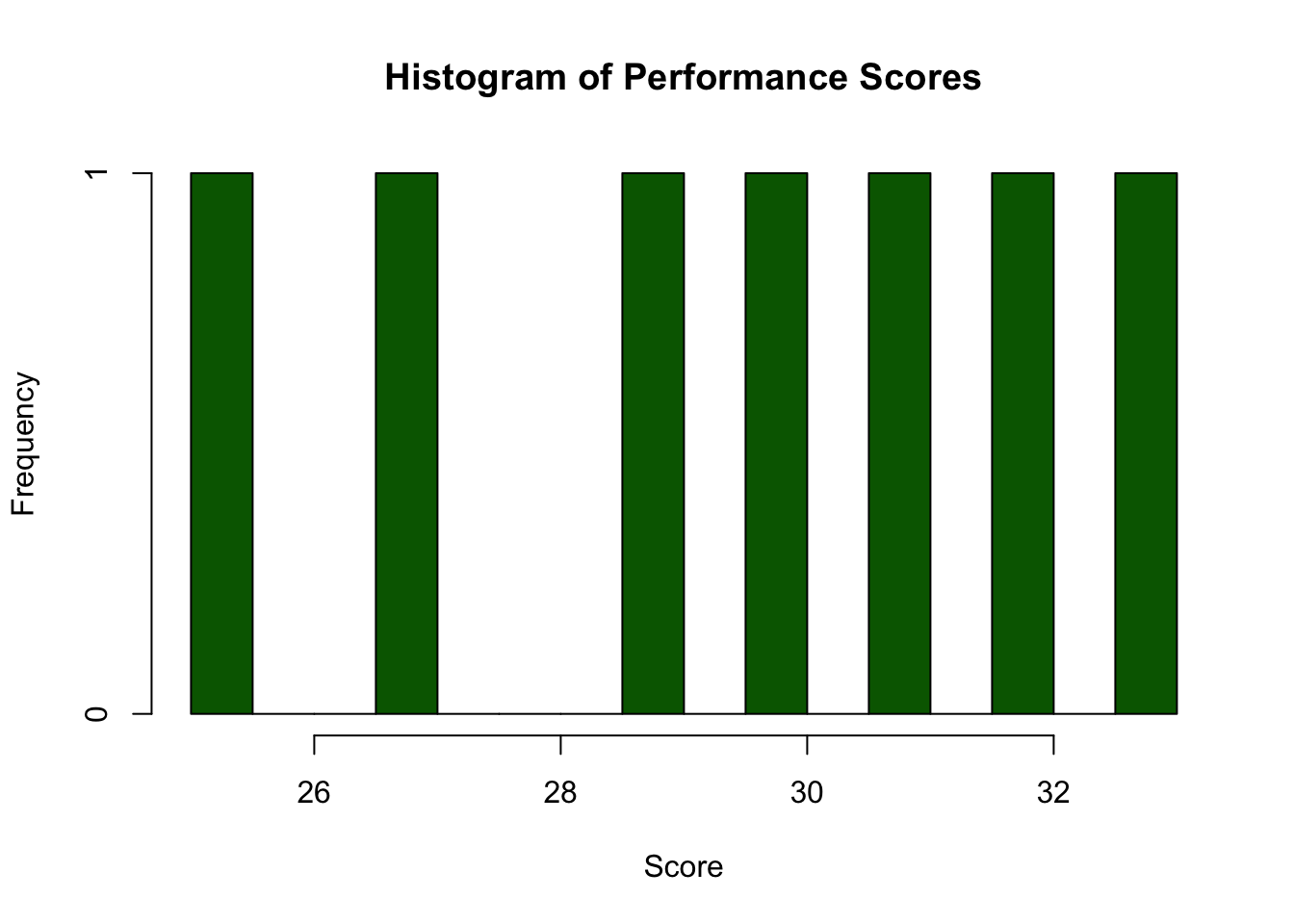
Here’s an example of data transformation on outliers using log transformation:
# Checking distributionhist(athlete_data$performance_score, main ="Histogram of Performance Scores", xlab ="Score", breaks =20, col ="darkgreen")
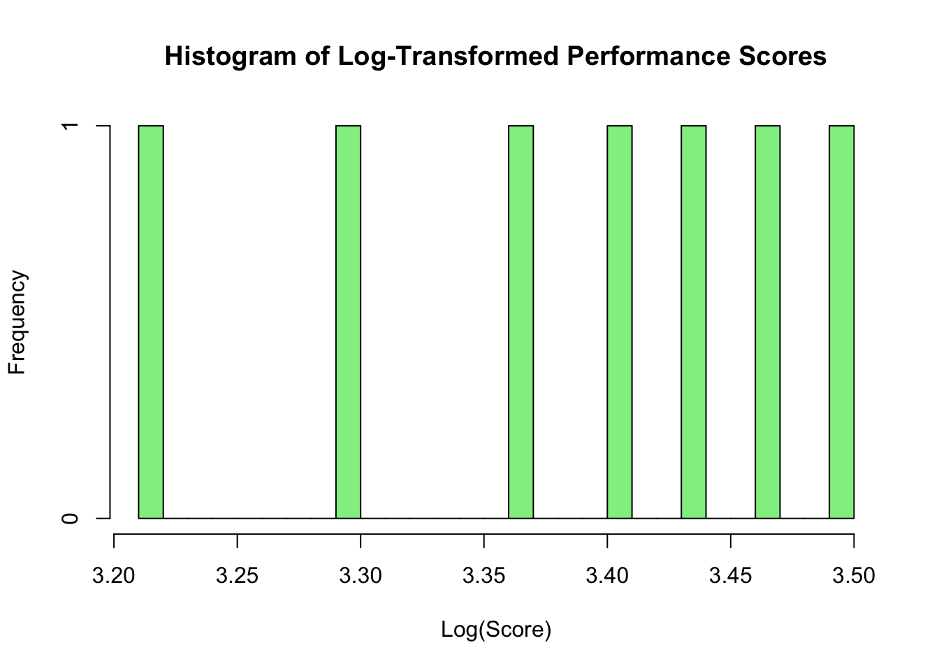
# Applying log transformation to reduce skewness caused by outliersathlete_data$transformed_score <-log(athlete_data$performance_score)# Visualise transformed datahist(athlete_data$transformed_score, main ="Histogram of Log-Transformed Performance Scores", xlab ="Log(Score)", breaks =20, col ="lightgreen")
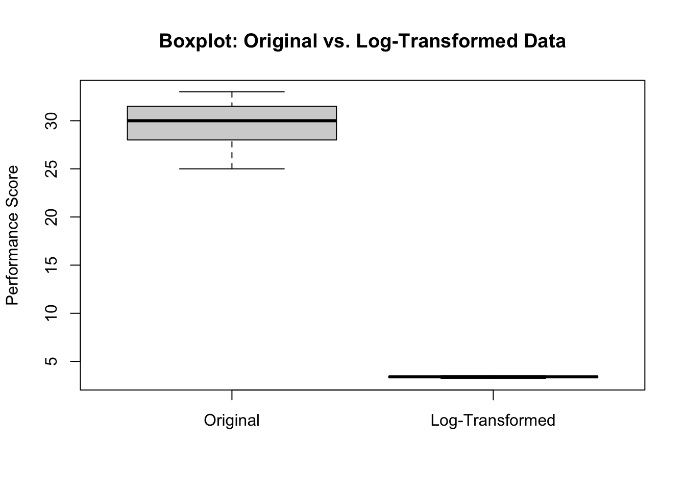
# Show how transformation has affected distribution and impact of outliersboxplot(athlete_data$performance_score, athlete_data$transformed_score,names =c("Original", "Log-Transformed"),main ="Boxplot: Original vs. Log-Transformed Data",ylab ="Performance Score")
rm(outliers)
72.4 Data normalisation
Theory
Data normalisation is a preprocessing step that aims to adjust the values in the dataset to a common scale without distorting differences in the ranges of values or losing information.
In ML, normalisation is crucial because it ensures that each feature contributes equally to the analysis, preventing bias towards variables with higher magnitude.
Especially in algorithms that compute distances or assume normality, such as k-means clustering or neural networks, normalisation can significantly improve performance.
There are several methods to normalise data, with min-max scaling being one of the most common. This method rescales the feature to a fixed range, usually 0 to 1. By doing this, you can ensure that each feature influences the model to an equal degree, enhancing the algorithm’s convergence and accuracy.
Demonstration
I need to normalise a dataset of a basketball players’ height and weight.
# Sample basketball players' height and weightset.seed(123)player_ids <-1:50heights_cm <-round(rnorm(50, mean =200, sd =10),1) # Heights centimetersweights_kg <-round(rnorm(50, mean =100, sd =15),1) # Weights kilogramsbasketball_data <-data.frame(player_ids, heights_cm, weights_kg)# Min-max normalisation functionmin_max_normalisation <-function(x) {return ((x -min(x)) / (max(x) -min(x)))}# Apply normalisation to height and weightbasketball_data$norm_heights <-min_max_normalisation(basketball_data$heights_cm)basketball_data$norm_weights <-min_max_normalisation(basketball_data$weights_kg)# View normalised datahead(basketball_data)
As observed earlier in the module, data standardisation is an important preprocessing step in ML. It involves transforming data to have a mean of zero and a standard deviation of one.
This process, often called ‘z-score normalisation’, ensures that each feature contributes equally to the analysis and helps in comparing measurements that have different units or scales.
Why is it important?
Equal Contribution: Without standardisation, features with larger scales dominate those in smaller scales when machine learning algorithms calculate distances.
Improved Convergence: In gradient descent-based algorithms (such as neural networks), standardisation can accelerate the convergence towards the minimum because it ensures that all parameters are updated at roughly the same rate.
Prerequisite for Algorithms: Many ML algorithms, like SVM and k-nearest neighbors (KNN), assume that all features are centered around zero and have variance in the same order.
Performance Metrics: When evaluating models, especially those in sport where performance metrics can vary widely (e.g., time vs. distance), standardisation allows for a fair comparison across different events or units.
Demonstration
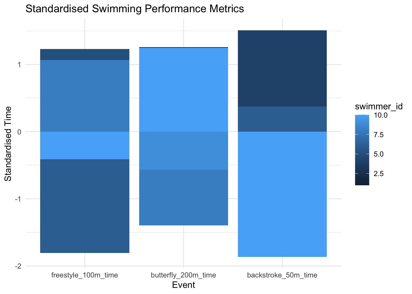
In this example, I’m going to standardise the performance metrics across different swimming events.
library(dplyr)
Attaching package: 'dplyr'
The following objects are masked from 'package:stats':

    filter, lag
The following objects are masked from 'package:base':

    intersect, setdiff, setequal, union
library(reshape2)set.seed(123)# Generating synthetic data for swimmers' performanceswimmers_data <-data.frame(swimmer_id =1:10,freestyle_100m_time =runif(10, 40, 55), # Time in secondsbutterfly_200m_time =runif(10, 110, 130), # Time in secondsbackstroke_50m_time =runif(10, 25, 35) # Time in seconds)head(swimmers_data)
# Visualisationlibrary(ggplot2)melted_data <-melt(standardised_data, id.vars ='swimmer_id')ggplot(melted_data, aes(x = variable, y = value, fill = swimmer_id)) +geom_bar(stat ="identity", position ="dodge") +labs(title ="Standardised Swimming Performance Metrics", x ="Event", y ="Standardised Time") +theme_minimal()
72.6 Dealing with imbalanced data
Theory
In machine learning, ‘imbalanced data’ refers to situations where the target classes are not represented equally.
For example, in a sports injury dataset, the number of non-injured instances might vastly outnumber the injured ones. This imbalance can bias predictive models toward the majority class, leading to poor generalisation on the minority class.
In the following dataset, there 190 observations with no injury, and only 10 with an injury.
library(caret)
Loading required package: lattice
library(DMwR2)
Registered S3 method overwritten by 'quantmod':
  method            from
  as.zoo.data.frame zoo
set.seed(123)# Generate synthetic datanum_athletes <-200speed <-rnorm(num_athletes, mean =25, sd =5) # Speed in km/hagility <-rnorm(num_athletes, mean =30, sd =7) # Agility measurementinjury <-c(rep(0, 190), rep(1, 10)) # Binary injury status, imbalancedathletes_data <-data.frame(speed, agility, injury)# View imbalance in the datasettable(athletes_data$injury)
  0   1
190  10
Synthetic data generation
One way of dealing with this is to use SMOTE (synthetic minority over-sampling technique) to generate synthetic data for the minority class.
Note: the previous library for this has been deprecated and the following code is not working properly
# Apply SMOTE to balance the dataset.seed(123)library(performanceEstimation)athletes_data_smote <-smote(injury ~ speed + agility, data = athletes_data, perc.over =2, k =5, perc.under=2)# View the new balancetable(athletes_data_smote$injury)
 0  1
40 10
Resampling
Another strategy is ‘resampling’, which can be used to adjust the distribution of classes within a dataset. Resampling aims to correct this imbalance, either by increasing the number of instances in the minority class (oversampling) or decreasing the number in the majority class (undersampling).
Here is an example of oversampling:
# Separate majority and minority classesdata_majority <- athletes_data[athletes_data$injury ==0, ]data_minority <- athletes_data[athletes_data$injury ==1, ]# Upsample minority classdata_minority_upsampled <- data_minority[sample(nrow(data_minority), 190, replace =TRUE), ]data_balanced <-rbind(data_majority, data_minority_upsampled)# View the new balancetable(data_balanced$injury)